Setting up a basic simulation

Summary

In this example, we see how to make StoSim run a simulation (a simple random walk) and generate plots from the resulting data. This example (like the others) can be found in the example folder of StoSim - I made comments in the code files when appropriate, especially for this basic example.

The two important things to look at are the configuration file and the simulation executable.

I’ll explain the most important steps here:

The basic example is a really simple simulation. We only want to simulate a random walk, run it several times and then plot the average outcome as well as maxima and minima for each run.

The Main Configuration File

This is the configuraton file for the basic simulation. We’ll look at all parts separately here - however, there is also a full reference of all possible configuration settings at Main configuration.

[meta]

We first take the opportunity to note some general information about our simulation: name and who is the maintainer.

# general simulation information
[meta]
# Name of your simulation
name:basic_sim
# The person who is responsible for this simulation
maintainer:Nicolas Hoening

[control]

We then describe how it should be run. What code should it call, how often should each configuration run, and should we distribute the runs on other computers. Our simulation executable is main.py and we’ll discuss it next. We run 5 times and are only doing it locally (we mention remote support in Using subsimulations). We also note that we use the tab delimiter (‘\t’) to separate between columns when we write log data (the default value is a comma, but the tab is also very common).

# which script to call for each run
executable:./main.py
# how often the same configuration should be run
runs:5
# default scheduler is fjd, but you can set it to pbs
scheduler: fjd
# the delimiter your simulation uses to separate values in its logs,
# defaults to comma (,) if you leave this setting away
delimiter:\t 

Note

Your executable will run under /bin/sh.

[params]

Then, we can add parameters specific to our simulation. That is, we mention parameters that will be used by the executable and tell StoSim to pass them on. This is simple in this case, we only specify how long our simulation should run: 500 timesteps.

[params]
# Parameters to your simulation (whichever you need)
# if you want more than one setting for a parameter, give a comma-separated list
steps:500

[plot-settings] and [figure<i>]

The rest of the configuration is spent with setting up a plot. You can specify several figures with each one or more plots (look out for the numbering).

We return to this below in Using the data: Making Plots and show the configuration relevant to our example there.

There is also a complete reference on settings for plots.

The Executable

Then, we need an executable. All your executable needs to do is read a configuration file StoSim hands it and write its output into a file which StoSim names. That is all there is to know about StoSim as far as your executable is concerned!

Below is the Python file from the basic example - it uses a lot of comments to explain what it is doing.

Note

Note that the executable doesn’t have to be a Python script. All you need to provide is any code that is executable (e.g. a Java, C or Perl script) and have it write its logs to the file with the name provided by StoSim.

#!/usr/bin/python
"""
Example stosim simulation runner,
showing very basic usage by conducting random walks

The only thing actually needed is a __main__ block (see bottom), so that this
script is callable from the command line.
The rest of this file shows how onfiguration files can be used and log files
be written. Pointers to both are supplied by StoSim.

Note that because StoSim calls this script in a system call
(like you would from a command line), this example could also be a Java file*.
The point is, your simulation doesn't have to be written in Python.
All it should do is read a config file and write to a log file.

* which you would need to precompile, of course
"""
try:
    import configparser
except ImportError:
    import ConfigParser as configparser  # for py2
import random
import sys


if __name__ == '__main__':
    '''
    This gets called by stosim for each run, since the name of this script
    was named in stosim.conf - StoSim will pass to it:
    (1) the name of the log file
    (2) the name of the conf file
    which are specific to this run.
    '''

    # open the conf file for this run with the standard Python way
    conf = configparser.ConfigParser()
    conf.read(sys.argv[1])
    # open the log StoSim says we should write to when we run this job
    log = open(conf.get('stosim', 'logfile'), 'w')

    # The parameters from the conf for this run can be accessed like this
    max_step = conf.getint('params', 'steps')

    val = 0
    random.seed()
    for step in range(1, max_step+1):
        dbl = random.random()
        if dbl > .5:
            val += 1
        else:
            val -= 1
        # we write two columns per row: step and value
        log.write("%d\t%d\n" % (step, val))
    log.flush()
    log.close()

Note

Note that we use the tab (\t) here to separate values, just as we told StoSim above.

Note

Note also that you can write comments in the logs (here: first line). Be sure to indicate comments with a starting ‘#’

Using the data: Making Plots

So we have now an simulation and it gets run by StoSim and it writes to log files. What do we do with them? Let’s make nice graphs! StoSim organizes all its log files in the data folder. For each configuration, log files are put into a subfolder whose name contains all parameter settings. We have only one possible setting now, so in examples/basic/data we now find the folder _steps500, containing five log files (Why five? We told StoSim to run each setting five times in the configuration).

Note

You could add further runs to your data. Use the --more command to add to your current data collection (see the example Using stochastic features).

General plot-settings

General settings of plots can be in the main configuration file or, for convenience, be put into the subsimulation files (see the next example Using subsimulations). Those settings can also be set per figure. Settings per figure overwrite plot-settings in subsimulations, which overwrite the plot-settings in the main configuration.

The first four settings are of purely cosmetic nature, while the fifth is really interesting when we discuss line plots below - in essence, we’re telling StoSim here not to draw vertical error bars.

[plot-settings]
# put general settings for plots you want to generate here.
# You can also do that per-figure
use-colors:1
line-width:6
font-size:22
infobox-pos: bottom right
use-y-errorbars:0

Settings per figure

Let’s first look at the settings per figure: name, x-label and y-label seem obvious. The y-range setting is dependent on what values you expect or want to see on the y-axis. We set the xcol to 1, since we wrote the step number in column 1 and the values in column 2.

Note

Note that all plots in each figure use the same x-axis.

[figure1]
# Name of figure: no spaces!
name: randomwalk_plot_1
# All the plots on one figure shoulod share the same xcolumn
xcol: 1
# The range of y-values you expect in the plots (e.g. [0:100)]
y-range: [-70:70]
#x-range: [0:500]
# names of axis
x-label: iteration
y-label: value

There can be many figures, each having one or more plots (numerate the options consistently, i.e. figure1, figure2, figure3 and plot1, plot2, plot3).

Settings per plot

Now pay attention to the plots descriptions, where each dataset which is plotted on the figure is described. StoSim can do two kinds of plots for you, line- and scatterplots, both of which are used in the example below.

# plot description(s): You need at least _name (no whitespace), _type (scatter or line) and _ycol. 
# In addition, list parameter settings in order to narrow down the dataset this graph should be about
plot1: _name:the_walk, _type:line, _ycol:2
plot2: _name:peaks, _type:scatter, _ycol:2, _select:max_y
plot3: _name:lows, _type:scatter, _ycol:2, _select:min_y

Settings to narrow down data

For each plot, you can specify name-value pairs (where the names refer to parameter names from the params section (see above). With this, you narrow down the dataset used for making the plot and this is also why StoSim puts all parameter settings in the data folder names containing the log files, so it can easily pick the ones it needs to collect data from.

In the current example figure, we have only one parameter (steps) with only one setting (500) - we could add steps:500 to the plot descriptions but that would still select all five files and thus change nothing. Thus, we do not use this feature in this example - we plot data from all five files we generated. The next example (see Using subsimulations) is a little bit more sophisticated in this regard.

StoSim-specific settings

In addition to that, there are stosim-specific settings per plot (to set them apart from parameters, they all start with an underscore).

• _name (Required) Each plot needs a name to identify it on the figure.
• _type (Required) StoSim currently supports two plot types - line and scatter. We’ll use both of them in a minute.
• _ycol (Required) This number indicates which column of your log files should be plotted on the y-axis. We wrote the values in column 2, so we take column 2 here as the y xolumn.
• _select This refers to a method to pick specific valued from the log files. We also used this in our figure, so we’ll discuss it below.

Selecting type and data

StoSim supports two types of plots and they both differ in their approach to data selection and preparation.

If you tell stosim to produce a line plot, it will average over all log files that are in matched data-folders and show the averages on a line. While doing so, it can automatically add error bars to the plot, showing the standard deviation in the data. This is the use-y-errorbars - setting which is for this example set to 0 (meaning no, where 1 would mean yes).

If you tell StoSim to produce a scatter plot, it will merely put all <x,y> data points on the figure. The interesting part is that you may want to select certain data points instead of plotting all of them (we already produce 5 * 500 = 25000 points in this example). We use the optional _select directive here to say that for each run StoSim made on our simulation, we want to select only one value - the maximal number which the random walk encountered and also the minimal (before you ask, StoSim currently has max-x, max-y, min-x, min-y and last. More are possible and I certainly want custom selectors).

Let’s now run the simulation with

$ stosim --folder examples/basic/

This is what I see on the terminal:

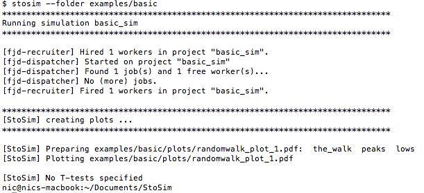
The terminal during a run of the basic example

You should now find a folder called data/_steps500. There, all the log files have been written. The folder name _steps500 indicates the parameter settings used in those runs (and in this simple example, we only have parameter with one setting).

Here is the plot which should be found in the examples/basic/plots directory if everything went well:

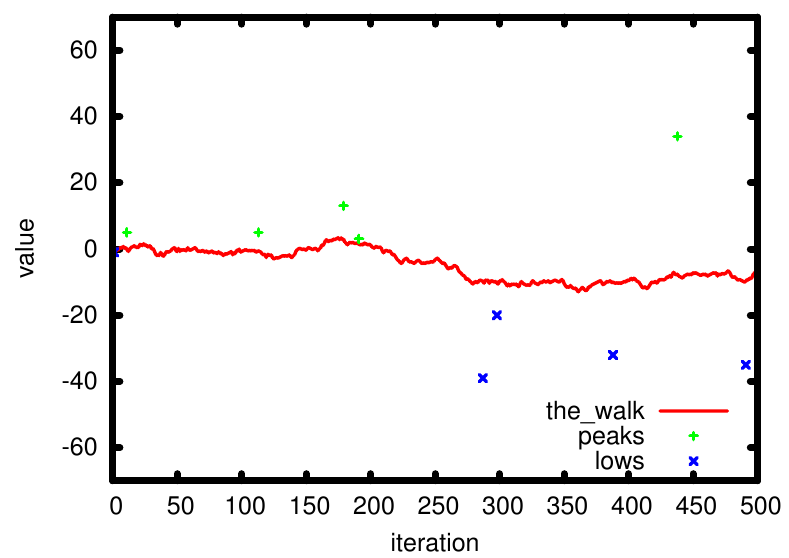
The plot created by the basic example

So we note that the average of five runs is visible between 10 and -10, but the actual maxima and minima range between 40 and -40, respectively. Otherwise, this example is not very useful scientifically :) Feel free to play with it. One could increase the number of runs to see the effect on the line. We will do that when we return to the random-walk example to discuss Using stochastic features.

This concludes the first tutorial - I hope it helped a little to explain how to use StoSim.